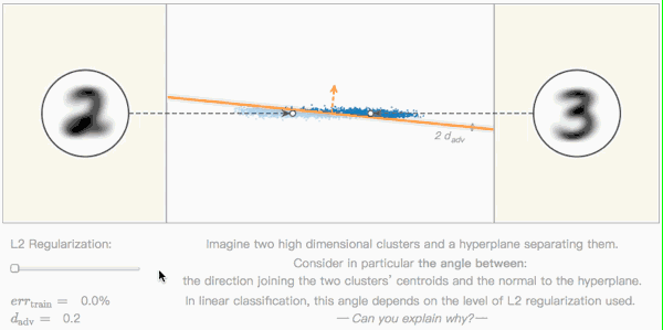
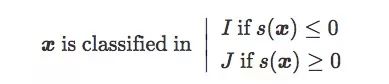
Editor's note: As shown in the figure below, this is a very basic classification problem: there are two high-dimensional clusters (two clusters of blue dots) in the space, and they are separated by a hyperplane (orange line). The two white dots represent the centroids of the two clusters, their Euclidean distance to the hyperplane determines the performance of the model, and the orange dashed line is their vertical direction.
In this type of linear classification problem, by adjusting the level of L2 regularization, we can continuously adjust the vertical angle. But can you explain why this is?
Many studies have confirmed that deep neural networks are easily affected by adversarial examples. By adding some subtle disturbances to the image, the classification model will suddenly face blindness and begin to refer to cats as dogs and males to females. As shown in the figure below, this is an American actor face classifier. After inputting a normal Steve Carell image, the probability that the model thinks the photo is him is 0.95. But when we added a little bit of material to his face, he became the actress Zooey Deschanel in the eyes of the model.
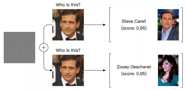
This result is worrying. First, it challenges a basic consensus that the good generalization of new data and the robustness (robustness) of the model to small disturbances are mutually reinforcing. The above figure makes this statement untenable. Second, it poses a potential threat to real-world applications. In November last year, MIT researchers added disturbances to 3D objects and successfully allowed the model to classify turtles as guns. In view of these two reasons, understanding this phenomenon and improving the robustness of neural networks has become an important research goal of the academic community.
In recent years, some researchers have explored several methods, such as describing phenomena, providing theoretical analysis, and designing more powerful structures. Adversarial training has now become a new regularization technique. Unfortunately, none of them can fundamentally solve this problem. Faced with this difficulty, a feasible way of thinking is to start from the most basic linear classification to gradually decompose the complexity of the problem.
Toy problem
In linear classification problems, we generally think that adversarial disturbances are dot products in high-dimensional spaces. In this regard, a very common saying is: we can make a large number of infinitely small changes to the input in high-dimensional problems, so that the output changes dramatically. But this argument is actually problematic. In fact, when the classification boundary is close to the data manifold, the adversarial sample still exists-in other words, it is independent of the image space dimension.
Modeling
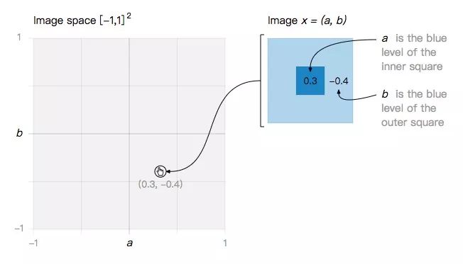
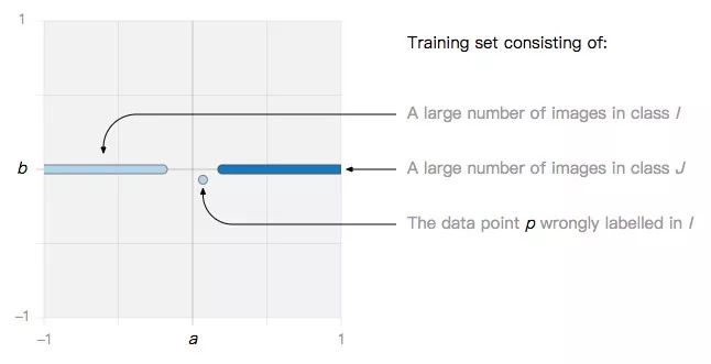
Let's start with a minimal toy problem: a two-dimensional image space, where each image is a function of a and b.
In this simple image space, we define two types of images:
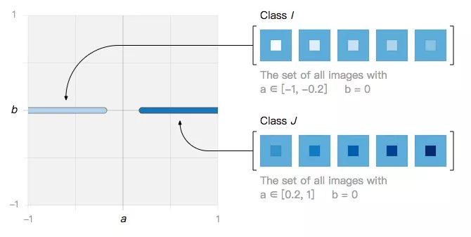
They can be classified by countless linear classifiers, such as Lθ in the figure below:
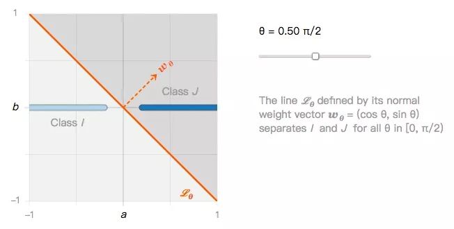
From this we can ask the first question: if all linear classifiers can classify class I images and class J images well, can they also classify image disturbances equally robustly?
Projection and mirroring
Assuming that x is an image in I, its shortest distance from the class J image is its projection to the classification boundary, that is, the vertical distance from x to Lθ:
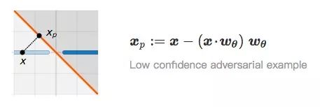
When x and xp are very close, we regard xp as an adversarial example of x. Relating to the first question, obviously, the confidence that xp is classified as I is very low and not robust. So are there any adversarial examples with high confidence? In the figure below, we find the mirror image xm of x in J based on the previous distance:
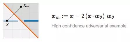
It is not difficult to understand that the distance between x and xm to the classification boundary is the same, and their classification confidence should also be the same.
Build a function about θ based on mirroring
Let's go back to the toy problem before. With the image x and its mirror image xm, we can construct a function containing θ accordingly.
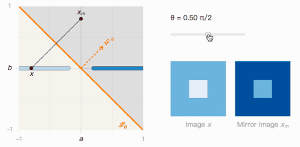
As shown in the figure above, the distance from x to xm depends on the angle θ of the classification boundary. Let's observe its two extreme values:
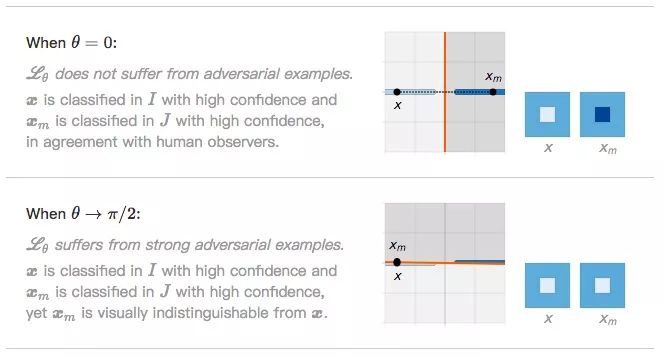
When θ=0, Lθ is not affected by adversarial samples. The confidence that x is classified as I is very high, and the confidence that xm is classified as J is also very high, we can easily distinguish the two.
When θ→π/2, Lθ is obviously affected by the adversarial sample. The confidence that x is classified as I is high, and the confidence that xm is classified as J is also high, but they are almost indistinguishable visually.
This brings up the second question: if Lθ is tilted more severely, the probability of existence of adversarial samples is higher, then what is actually affecting Lθ?
Overfitting and L2 regularization
For this problem, the hypothesis of this article is standard linear models, such as SVM and logistic regression, which are excessively skewed because of overfitting the noise data in the training set. The theoretical results of Huan Xu et al. in the paper Robustness and Regularization of Support Vector Machines support this hypothesis and believe that the robustness of the classifier is related to regularization.
To prove this is not difficult, let's do an experiment: Can L2 regularization weaken the influence of adversarial examples?
Suppose there is a noisy data point p in the training set:
If the algorithm we use is SVM or logistic regression, these two situations may be observed in the end.
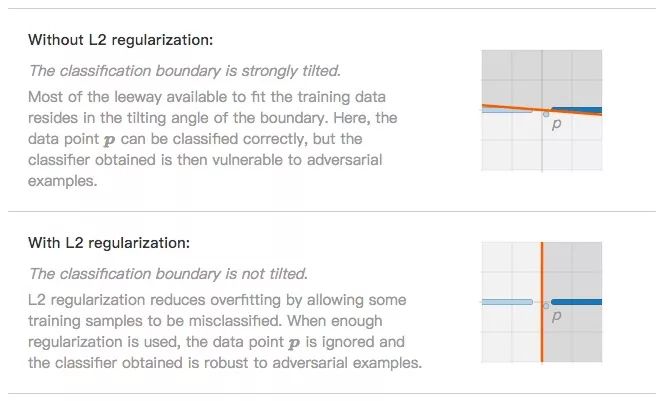
The classification boundary is severely inclined (no L2 regularization). In order to fit the data points as much as possible, the classification boundary will try to tilt so that the model can finally accurately classify p. At this time, the classifier is over-fitting and is more susceptible to the influence of adversarial samples.
The classification boundary is not inclined (L2 regularization). The idea of ​​L2 regularization to prevent overfitting is to allow a small part of the data to be classified incorrectly, such as noise data p. After ignoring it, the classifier is more robust in the face of adversarial examples.
Seeing this, some people may have objections: The above data is two-dimensional, what does it have to do with high-dimensional data?
Adversarial examples in linear classification
We have drawn two conclusions before: (1) The closer the classification boundary is to the data manifold, the easier it is for adversarial samples to appear; (2) L2 regularization can control the tilt angle of the boundary. Although they are all proposed based on two-dimensional image space, they are actually true for general situations.
Scaling loss function
Let's start with the simplest. L2 regularization is to add a regularization term after the loss function. Unlike L1, which puts the weight to 0, the weight vector of L2 regularization is continuously decreasing, so it is also called weight decay.
Modeling
Let I and J be the two types of images in the high-dimensional image space Rd, and C is the hyperplane boundary output by the linear classifier, which is related to the weight vector w and the bias term b. x is a picture in Rd, the original score from x to C is:
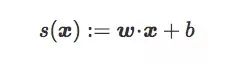
This original score is actually the signed distance of x with respect to C (signed distance, signed):
Suppose there is a training set T containing n pairs (x, y), where x is an image sample, when x∈I, y=-1; when x∈J, y=1. The following are three distributions of T:

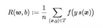
The expected risk R(w,b) of the classifier C is the average penalty on the training set T:
Under normal circumstances, when we train a linear classifier, we will use the appropriate loss function f to find the weight vector w and the bias term b to minimize R(w, b). In general binary classification problems, the following are three loss functions worth paying attention to:

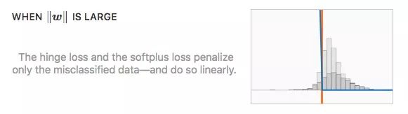
As shown in the figure above, for the first loss function, the expected risk of the classifier is its classification error rate. In a sense, this loss function is the most ideal, because we only need to minimize the error to achieve the goal. But its disadvantage is that the derivative is always 0, and we cannot use gradient descent on this basis.
In fact, the above problems have now been solved. Some linear regression models use improved loss functions, such as the hinge loss of SVM and the softplus loss of logistic regression. They no longer continue to use a fixed penalty term on the misclassified data, but use a strictly decreasing penalty term. As a cost, these loss functions will also bring side effects to the correctly classified data, but in the end it can be guaranteed to find a more accurate classification boundary.
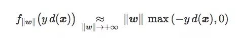
Scaling parameter ‖w‖
When introducing the symbol distance s(x) before, we did not elaborate on its scaling parameter w. If d(x) is the Euclidean distance from x to C, we have:

Therefore, ‖w‖ can also be regarded as the scaling parameter of the loss function:
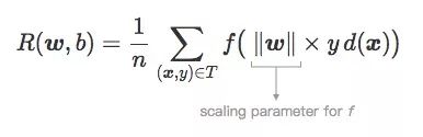
That is: f‖w‖:z→f(‖w‖×z).
It can be found that this scaling has no effect on the first loss function mentioned before, but it has a dramatic effect on hinge loss and softplus loss.

It is worth noting that for the extreme values ​​of the scaling parameters, the last two loss functions change the same.
More precisely, both loss functions satisfy:
For convenience, we define the misclassified data as:
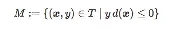
So the expected risk can be rewritten as:
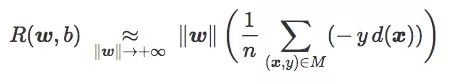
This expression contains a concept we call "error distance":

It is positive and can be interpreted as the average distance for each training sample to be misclassified by C (zero contribution to correctly classified data). It is related to training error, but not exactly the same.
Finally, we can get:
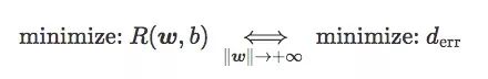
In other words, when "w" is large enough, minimizing the expected risk of hinge loss and softplus loss is equivalent to minimizing the error distance, that is, minimizing the error rate on the training set.
summary
To sum up, by adding a regularization term after the loss function, we can control the value of ‖w‖ and output the regularized loss.
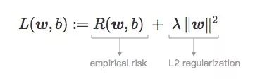
A smaller regularization parameter λ will make ‖w‖ increase out of control, and a larger λ will make ‖w‖ decrease.
In summary, the two standard models used in linear classification (SVM and logistic regression) strike a balance between two goals: they minimize the error distance when the regularization parameter is low, and maximize the adversarial distance when the regularization coefficient is high.
Confrontation distance and tilt angle
Seeing this, we have come into contact with a new term-"antagonistic distance"-a measure of the robustness of adversarial disturbances. Like the previous two-dimensional image space example, it can be expressed as a function containing a single parameter, which is the angle between the classification boundary and the nearest centroid classifier.
For the training set T, if we divide it into TI and TJ according to image categories I and J, we can get:
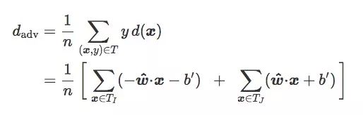
If TI and TJ are equal (n=2nI=2nJ):

Let the centroids of TI and TJ be i and j respectively:
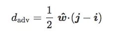
Now there is a centroid classifier closest to the classification boundary, and its normal vector is z^=(j−i)/‖j−i‖:
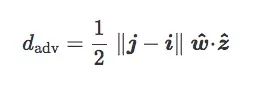
Finally, we call the plane containing w^ and z^ the inclined plane of C, and we call the angle θ between w^ and z^ the inclination angle of C:
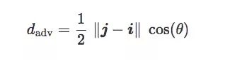
The geometric meaning of this equation is shown in the figure below:

Based on the above calculations, on a given training set T, if the distance between two centroids ‖j−i‖ is a fixed value, the confrontation distance dadv depends only on the tilt angle θ. In layman's terms:
When θ=0, the adversarial distance is the largest and the impact of the adversarial sample is the smallest;
When θ→π/2, the adversarial distance is the smallest, and the adversarial sample has the greatest impact on the classifier.
Final words
Although adversarial samples have been studied for many years, and although they are of great significance to the field of machine learning in theory and practice, the research on it in the academic field is still very limited, and it is still a mystery to many people. This article gives the generation of adversarial examples under the linear model, and hopes to provide some insights to newcomers who are interested in this aspect.
Unfortunately, the reality is not as simple as the article describes. As the data set becomes larger and the neural network continues to deepen, the adversarial examples are becoming more and more complex. In our experience, the more nonlinear factors the model contains, the more useful the weight attenuation seems to be. This discovery may only be at a shallow level, but the deeper content will be solved by new people who are constantly emerging. What is certain is that if we want to give a convincing solution to this difficulty, we need to witness the birth of a new revolutionary concept in deep learning.
Our company specializes in the production and sales of all kinds of terminals, copper terminals, nose wire ears, cold pressed terminals, copper joints, but also according to customer requirements for customization and production, our raw materials are produced and sold by ourselves, we have their own raw materials processing plant, high purity T2 copper, quality and quantity, come to me to order it!
Copper Connecting Terminals,Cable Lugs Insulated Cord End Terminals,Pvc Insulated Cord End Terminal,Cable Connector Insulated Cord End Terminal
Taixing Longyi Terminals Co.,Ltd. , https://www.lycopperterminals.com