In this issue of AI Adventure, Yufeng will lead us to follow the best practices we shared before and try to walk through the entire process of machine learning. The workload is a bit big, but smart you should be fine.
Training models using MNIST data* is often seen as a “Hello World†example in the machine learning world (training handwritten character recognition models using standard MNIST data), and today we follow Yufeng to use more “fashionable†data to turn on the machine Learning Hello World.
* Paragraph Note: MNIST is a dataset of handwritten digital images, each of which is marked by an integer. It is mainly used for performance benchmarking of machine learning algorithms.
"Middle" Machine Learning
Zalando (an e-commerce company from Germany) is determined to make MNIST "fire" again. Some time ago Zalando's research department released a data set called Fashion-MNIST. This is a data set that has the same format as MNIST. The only difference is that handwritten characters have been replaced with clothing, shoes, satchels, and so on. It still has 10 categories and the image is still 28x28 pixels.
See more about the Fashion-MNIST dataset on GitHub (in Chinese):
https://github.com/zalandoresearch/fashion-mnist/blob/master/README.zh-CN.md

Let's train a model together and use it to identify the category of clothing that belongs to it!
Linear Classifier
Let's start by building a linear classifier and see how it works. As always, we use TensorFlow's evaluator framework (linked below for paragraphs) to simplify programming and maintenance. Recall that we will go through the process of loading data, creating a classifier, and running training and evaluation. In addition, some predictions will be made directly with the local model. The official documentation refers to:
Https://tensorflow.google.com/get_started/get_started_for_beginners?hl=en
Let's start by creating a model. We first convert the image in the dataset from a 28x28 pixel arrangement to a 1x784 form and then call it the feature column pixels. This operation is similar to AIA's third issue: It is easy to figure out the flower_features that appear in the iris identification model without mathematics knowledge.
Feature_columns = [tf.feature_column.numeric_column( "pixels", shape=784)]classifier = tf.estimator.LinearClassifier( feature_columns=feature_columns, n_classes=10, model_dir=logdir)
The next step is to create a linear classifier. We have 10 categories that need to be marked, not three of the previous Iris cases.
To start training, we need to configure the data set and input function. TensorFlow has built-in functions that accept a NumPy array for generating input functions, and we use it here to simplify it.
Tf.estimator.inputs.numpy_input_fn( x={'pixels': X}, y=Y, batch_size=batch_size, num_epochs=epochs, shuffle=shuffle) DATA_SETS = input_data.read_data_sets( "/tmp/fashion-mnist")
Then use the input_data module to load the dataset and point the function parameter to the location where the dataset was downloaded.
Then combine the classifier, input function, and data set by calling classifier.train().
Classifier.train(input_fn=train_input_fn, steps=num_steps)accuracy_score = classifier.evaluate(input_fn=eval_input_fn)['accuracy']
Finally, we conduct an assessment to see how the model performs. When using the classic MNIST data set, this model often gets about 91% accuracy. Then, because the fashion version of MNIST has a more complex data set, it is only slightly more than 80% accurate, and sometimes even lower.
How can we improve it? For example, AIA Sixth: It is better to go through the deep neural network to recognise what the Estimator mentioned.
Turn to depth model
Switching to the DNNClassifier is just a matter of replacing the line of code. Now restart the training and then evaluate to see if the depth model will be better than linear.
Classifier = tf.estimator.DNNClassifier( feature_columns=feature_columns, n_classes=10, hidden_units=[100, 75, 50], model_dir=logdir )
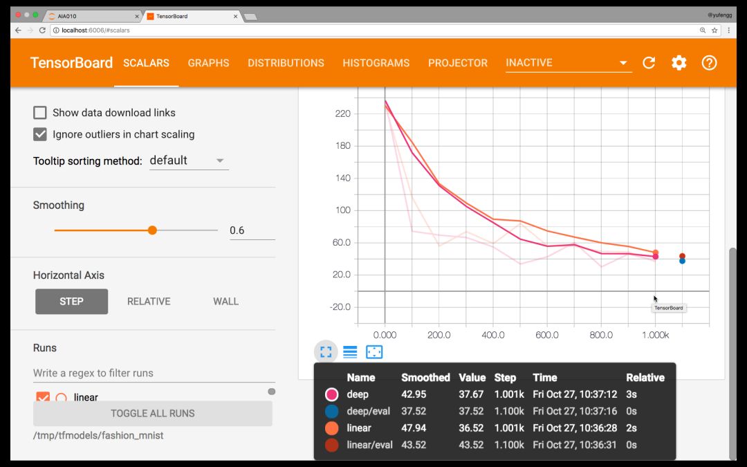
Just as in the fifth issue: As discussed in TensorBoard's Visualization of Models, we should use TensorBoard to laterally compare two models.
Tensorboard --logdir=models/fashion_mnist/
Browser opens http://localhost:6006
TensorBoard
Looking at Tensorboard, it seems that the depth model is no better than the linear model! This is probably due to the inadequacy of fine-tuning of hyperparameters. See AIA Phase 2: Common Machine Learning Steps.
Looks like it's going to go all the way...
Maybe our model needs more to accommodate models that are so complex? Or should training be less? Let's try it. After repeated debugging of the micro-parameters, the distortion of the model is reduced to a breakthrough, and the precision obtained by the model is higher than that of the linear model.
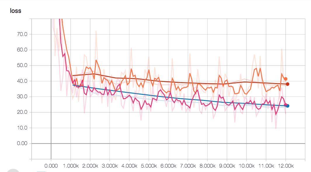
Depth model (blue vs. linear red line) distortion remains low
There are a few more steps in training before reaching this accuracy, but ultimately higher accuracy makes these efforts worthwhile.
It can be seen from the figure that the flat period of the linear model is earlier than the depth network. This is because depth models are more complex and they require longer training times.
At this point, the model almost meets our requirements. We can export it and generate a scalable fashion version of the MNIST classifier API. As for how to export, you can refer to the detailed steps given in the fourth period.
prediction
Let's quickly review how to use the evaluator to make predictions. To a large extent, it is like the way we train and evaluate; it is also a great advantage of the evaluator (framework) - a universally consistent function interface.
X = DATA_SETS.test.images[5000:5005]predict_input_fn = tf.estimator.inputs.numpy_input_fn( x={'pixels': X}, batch_size=1, num_epochs=1, shuffle=False) predictions = classifier.predict( Input_fn=predict_input_fn)
Note that we specify batch_size as 1, num_epochs as 1, and shuffle as false. This is because we want to predict one by one, one at a time, on all data. I selected five images for prediction from the data sets used in the assessment.
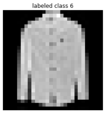
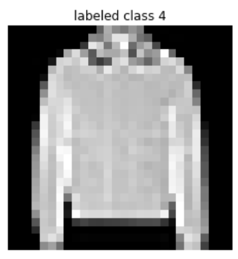
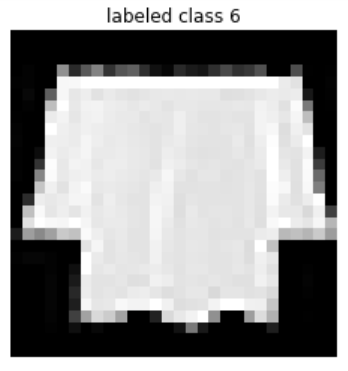
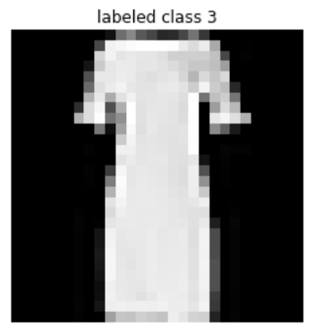
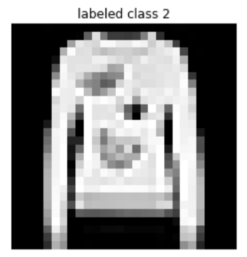
The reason I chose these 5 images is not only because they are in the middle, but also because two of these models are incorrect. Both should be shirts, but the model is considered to be the third is the package and the fifth is the coat. Thus, considering only the factor of the texture change of the image, you can see how challenging these samples are compared to hand-written numbers.
Next steps
You can see the code used to train and generate images in this share on this Gist (linked after paragraph). How is your model performing? What is the final parameter you adopted? Share it in the comments!
Https://gist.github.com/yufengg/2b2fd4b81b72f0f9c7b710fa87077145
Highlights
The next few issues will focus on the tools of the machine learning ecology to help you create your own operating procedures and toolchain. At the same time, it also shows more model architectures that can be used to solve machine learning problems. I am very much looking forward to continuing to analyze and answer for you in the following sharing! Before that, don't forget to use machine learning!
The Mining Transformer,Mining Transformer,Electric Power Transformer,Electric Transformer
SANON DOTRANSÂ Co., Ltd. , https://www.sntctransformer.com